Reading Planetary Computer Data using CQL2 filter extension

library(rstac)

Introduction

This tutorial will use the open-source package rstac to search data in Planetary Computer’s SpatioTemporal Asset Catalog (STAC) service. STAC services can be accessed through STAC API endpoints, which allow users to search datasets using various parameters such as space and time. In addition to demonstrating the use of rstac, the tutorial will explain the Common Query Language (CQL2) filter extension to narrow the search results and find datasets that meet specific criteria in the STAC API.

This tutorial is based on reading STAC API data in Python.

Reading data from STAC API

To access Planetary Computer STAC API, we’ll create a rstac query.

planetary_computer <- stac("https://planetarycomputer.microsoft.com/api/stac/v1")
planetary_computer
#> ###RSTACQuery
#> - url: https://planetarycomputer.microsoft.com/api/stac/v1
#> - params:
#> - field(s): version, base_url, endpoint, params, verb, encode

Listing supported properties in CQL2

CQL2 expressions can be constructed using properties that refer to attributes of items. A list of all properties supported by a collection can be obtained by accessing the /collections/<collection_id>/queryables endpoint. Filter expressions can use properties listed in this endpoint.

In this example, we will search for Landsat Collection 2 Level-2 imagery of the Microsoft main campus from December 2020. The name of this collection in STAC service is landsat-c2-l2. Here we’ll prepare a query to retrieve its queriables and make a GET request to the service.

planetary_computer |>
  collections("landsat-c2-l2") |> 
  queryables() |> 
  get_request()
#> ###Queryables
#> - properties
#>   - datetime
#>   - id
#>   - eo:cloud_cover
#>   - view:off_nadir
#>   - view:sun_azimuth
#>   - view:sun_elevation
#>   - landsat:wrs_row
#>   - landsat:wrs_path
#>   - landsat:scene_id
#>   - landsat:cloud_cover_land
#>   - landsat:collection_category
#>   - platform
#>   - instrument
#> - field(s): $schema, $id, type, title, properties

Searching with CQL2

Now we can use rstac to make a search query with CQL2 filter extension to obtain the items.

time_range <- cql2_interval("2020-12-01", "2020-12-31")
bbox <- c(-122.2751, 47.5469, -121.9613, 47.7458)
area_of_interest = cql2_bbox_as_geojson(bbox)

stac_items <- planetary_computer |>
  ext_filter(
    collection == "landsat-c2-l2" &&
      t_intersects(datetime, {{time_range}}) &&
      s_intersects(geometry, {{area_of_interest}})
  ) |>
  post_request()

In that example, our filter expression used a temporal (t_intersects) and a spatial (s_intersects) operators. t_intersects() only accepts interval as it second argument, which we created using function cql2_interval(). s_intersects() spatial operator only accepts GeoJSON objects as its arguments. This is why we had to convert the bounding box vector (bbox) into a structure representing a GeoJSON object using the function cql2_bbox_as_geojson(). We embrace the arguments using {{ to evaluate them before make the request.

items is a STACItemCollection object containing 8 items that matched our search criteria.

stac_items
#> ###STACItemCollection
#> - features (8 item(s)):
#>   - LC08_L2SP_046027_20201229_02_T2
#>   - LE07_L2SP_047027_20201228_02_T1
#>   - LE07_L2SP_046027_20201221_02_T2
#>   - LC08_L2SP_047027_20201220_02_T2
#>   - LC08_L2SP_046027_20201213_02_T2
#>   - LE07_L2SP_047027_20201212_02_T1
#>   - LE07_L2SP_046027_20201205_02_T1
#>   - LC08_L2SP_047027_20201204_02_T1
#> - assets: 
#> ang, atmos_opacity, atran, blue, cdist, cloud_qa, coastal, drad, emis, emsd, green, lwir, lwir11, mtl.json, mtl.txt, mtl.xml, nir08, qa, qa_aerosol, qa_pixel, qa_radsat, red, rendered_preview, swir16, swir22, tilejson, trad, urad
#> - item's fields: 
#> assets, bbox, collection, geometry, id, links, properties, stac_extensions, stac_version, type

Exploring data

A STACItemCollection is a regular GeoJSON object. It is a collection of STACItem entries that stores metadata on assets. Users can convert a STACItemCollection to a sf object containing the properties field as columns. Here we depict the items footprint.

sf <- items_as_sf(stac_items)

# create a function to plot a map
plot_map <- function(x) {
  library(tmap)
  library(leaflet)
  current.mode <- tmap_mode("view")
  tm_basemap(providers[["Stamen.Watercolor"]]) +
    tm_shape(x) + 
    tm_borders()
}

plot_map(sf)
#> tmap mode set to interactive viewing

Some collections use the eo extension, which allows us to sort items by attributes like cloud coverage. The next example selects the item with lowest cloud_cover attribute:

cloud_cover <- stac_items |>
  items_reap(field = c("properties", "eo:cloud_cover"))
selected_item <- stac_items$features[[which.min(cloud_cover)]]

We use function items_reap() to extract cloud cover values from all features.

Each STAC item have an assets field which describes files and provides link to access them.

items_assets(selected_item)
#>  [1] "ang"              "atran"            "blue"             "cdist"           
#>  [5] "coastal"          "drad"             "emis"             "emsd"            
#>  [9] "green"            "lwir11"           "mtl.json"         "mtl.txt"         
#> [13] "mtl.xml"          "nir08"            "qa"               "qa_aerosol"      
#> [17] "qa_pixel"         "qa_radsat"        "red"              "rendered_preview"
#> [21] "swir16"           "swir22"           "tilejson"         "trad"            
#> [25] "urad"

purrr::map_dfr(items_assets(selected_item), function(key) {
  tibble::tibble(asset = key, description = selected_item$assets[[key]]$title)
})
#> # A tibble: 25 × 2
#>    asset   description                       
#>    <chr>   <chr>                             
#>  1 ang     Angle Coefficients File           
#>  2 atran   Atmospheric Transmittance Band    
#>  3 blue    Blue Band                         
#>  4 cdist   Cloud Distance Band               
#>  5 coastal Coastal/Aerosol Band              
#>  6 drad    Downwelled Radiance Band          
#>  7 emis    Emissivity Band                   
#>  8 emsd    Emissivity Standard Deviation Band
#>  9 green   Green Band                        
#> 10 lwir11  Surface Temperature Band          
#> # … with 15 more rows

Here, we’ll inspect the rendered_preview asset. To plot this asset, we can use the helper function preview_plot() and provide a URL to be plotted. We use the function assets_url() to get the URL. This function extracts all available URLs in items.

selected_item$assets[["rendered_preview"]]$href
#> [1] "https://planetarycomputer.microsoft.com/api/data/v1/item/preview.png?collection=landsat-c2-l2&item=LC08_L2SP_047027_20201204_02_T1&assets=red&assets=green&assets=blue&color_formula=gamma+RGB+2.7%2C+saturation+1.5%2C+sigmoidal+RGB+15+0.55"

selected_item |> 
  assets_url(asset_names = "rendered_preview") |>
  preview_plot()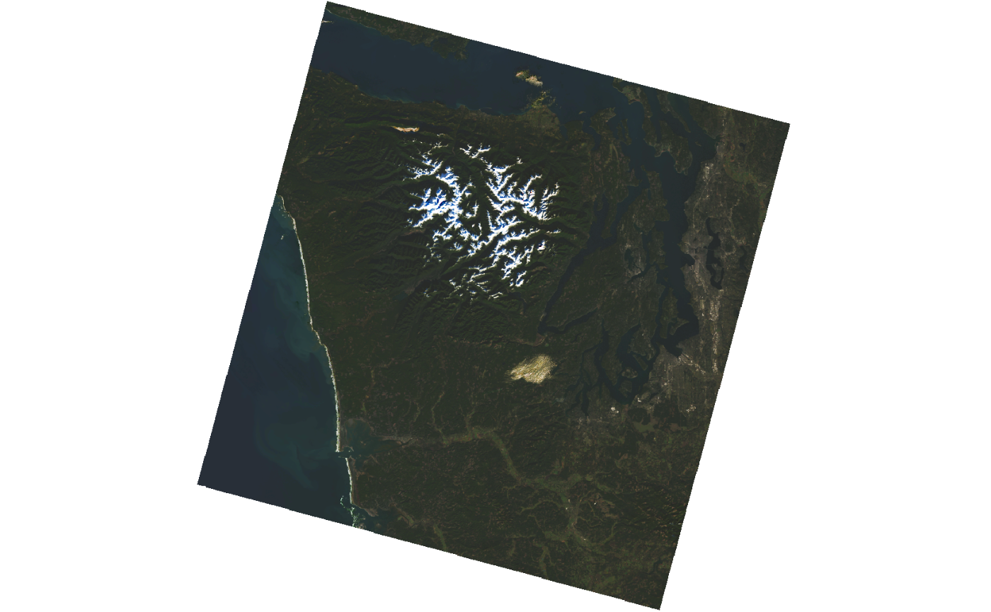

The rendered_preview asset is generated dynamically by Planetary Computer API using raw data. We can access the raw data, stored as Cloud Optimized GeoTIFFs (COG) in Azure Blob Storage, using the other assets. These assets are in private Azure Blob Storage containers and is necessary to sign them to have access to the data, otherwise, you’ll get a 404 (forbidden) status code.

Signing items

To sign URL in rstac, we can use items_sign() function.

selected_item <- selected_item |>
  items_sign(sign_fn = sign_planetary_computer())

selected_item |> 
  assets_url(asset_names = "blue") |>
  substr(1, 255)
#> [1] "https://landsateuwest.blob.core.windows.net/landsat-c2/level-2/standard/oli-tirs/2020/047/027/LC08_L2SP_047027_20201204_20210313_02_T1/LC08_L2SP_047027_20201204_20210313_02_T1_SR_B2.TIF?st=2023-01-20T20%3A00%3A48Z&se=2023-01-21T20%3A45%3A48Z&sp=rl&sv=2021"

Everything after the ? in that URL is a SAS token grants access to the data. See https://planetarycomputer.microsoft.com/docs/concepts/sas/ for more on using tokens to access data.

library(httr)
selected_item |> 
  assets_url(asset_names = "blue") |>
  httr::HEAD() |>
  httr::status_code()
#> [1] 200

The 200 status code means that we were able to access the data using the signed URL with the SAS token included.

Reading files

We can load up that single COG file using packages like stars or terra.

library(stars)
#> Loading required package: abind
#> Loading required package: sf
#> Linking to GEOS 3.9.1, GDAL 3.3.2, PROJ 7.2.1; sf_use_s2() is TRUE
selected_item |> 
  assets_url(asset_names = "blue", append_gdalvsi = TRUE) |>
  stars::read_stars(RasterIO = list(nBufXSize = 512, nBufYSize = 512)) |>
  plot(main = "blue")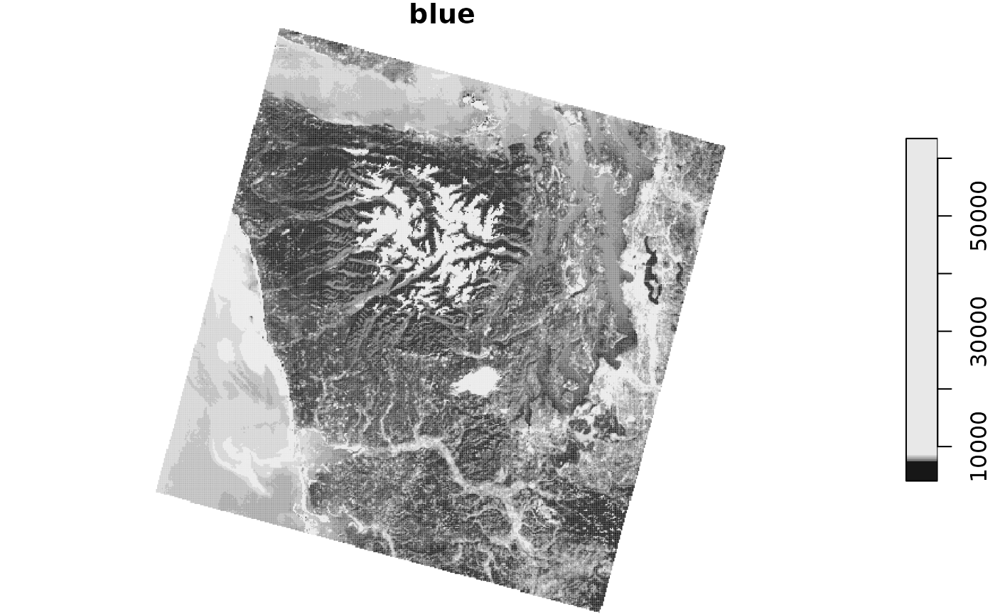

We used the assets_url() method with the append_gdalvsi = TRUE parameter to insert /vsicurl in the URL. This allows the GDAL VSI driver to access the data using HTTP.

Searching on additional properties

In the previous step of this tutorial, we learned how to search for items by specifying the space and time parameters. However, the Planetary Computer’s STAC API offers even more flexibility by allowing you to search for items based on additional properties.

For instance, collections like sentinel-2-l2a and landsat-c2-l2 both implement the eo STAC extension and include an eo:cloud_cover property. To filter your search results to only return items that have a cloud coverage of less than 20%, you can use:

stac_items <- planetary_computer |>
  ext_filter(
    collection %in% c("sentinel-2-l2a", "landsat-c2-l2") &&
      t_intersects(datetime, {{time_range}}) &&
      s_intersects(geometry, {{area_of_interest}}) &&
      `eo:cloud_cover` < 20
  ) |>
  post_request()

Here we search for sentinel-2-l2a and landsat-c2-l2 assets. As a result, we have images from both collections in our search results. Users can rename the assets to have a common name in both collections.

stac_items <- stac_items |>
  assets_select(asset_names = c("B11", "swir16")) |>
  assets_rename(B11 = "swir16")

stac_items |>
  items_assets()
#> [1] "swir16"

assets_rename() uses parameter mapper that is used to rename asset names. The parameter can be either a named list or a function that is called against each asset metadata. A last parameter was included to force band renaming.

Analyzing STAC Metadata

STACItem objects are features of STACItemCollection and store information about assets.

stac_items <- planetary_computer |>
  ext_filter(
    collection == "sentinel-2-l2a" &&
      t_intersects(datetime, interval("2020-01-01", "2020-12-31")) &&
      s_intersects(geometry, {{
        cql2_bbox_as_geojson(c(-124.2751, 45.5469, -123.9613, 45.7458))
      }})
  ) |>
  post_request()

stac_items <- items_fetch(stac_items)

We can use the metadata to plot cloud cover of a region over time, for example.

library(dplyr)
#> 
#> Attaching package: 'dplyr'
#> The following objects are masked from 'package:stats':
#> 
#>     filter, lag
#> The following objects are masked from 'package:base':
#> 
#>     intersect, setdiff, setequal, union
library(slider)
library(ggplot2)

df <- items_as_sf(stac_items)  |>
  dplyr::mutate(datetime = as.Date(datetime)) |>
  dplyr::group_by(datetime) |>
  dplyr::summarise(`eo:cloud_cover` = mean(`eo:cloud_cover`)) |>
  dplyr::mutate(
    `eo:cloud_cover` = slider::slide_mean(
      `eo:cloud_cover`, before = 3, after = 3
    )
  )

df |> 
  ggplot2::ggplot() +
  ggplot2::geom_line(ggplot2::aes(x = datetime, y = `eo:cloud_cover`))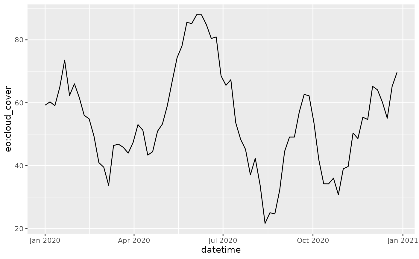

cql2_bbox_as_geojson() is a rstac helper function and it must be evaluated before the request. This is why we embraced it with {{. We use items_fetch() to retrieve all paginated items matched in the search.

Working with STAC Catalogs and Collections

STAC organizes items in catalogs (STACCatalog) and collections (STACCollection). These JSON documents contains metadata of the dataset they refer to. For instance, here we look at the Bands available for Landsat 8 Collection 2 Level 2 data:

landsat <- planetary_computer |>
  collections(collection_id = "landsat-c2-l2") |>
  get_request()

library(purrr)
purrr::map_dfr(landsat$summaries$`eo:bands`, tibble::as_tibble_row)
#> # A tibble: 22 × 5
#>    name   common_name description                                cente…¹ full_…²
#>    <chr>  <chr>       <chr>                                        <dbl>   <dbl>
#>  1 TM_B1  blue        Visible blue (Thematic Mapper)                0.49    0.07
#>  2 TM_B2  green       Visible green (Thematic Mapper)               0.56    0.08
#>  3 TM_B3  red         Visible red (Thematic Mapper)                 0.66    0.06
#>  4 TM_B4  nir08       Near infrared (Thematic Mapper)               0.83    0.14
#>  5 TM_B5  swir16      Short-wave infrared (Thematic Mapper)         1.65    0.2 
#>  6 TM_B6  lwir        Long-wave infrared (Thematic Mapper)         11.4     2.1 
#>  7 TM_B7  swir22      Short-wave infrared (Thematic Mapper)         2.22    0.27
#>  8 ETM_B1 blue        Visible blue (Enhanced Thematic Mapper Pl…    0.48    0.07
#>  9 ETM_B2 green       Visible green (Enhanced Thematic Mapper P…    0.56    0.08
#> 10 ETM_B3 red         Visible red (Enhanced Thematic Mapper Plu…    0.66    0.06
#> # … with 12 more rows, and abbreviated variable names ¹center_wavelength,
#> #   ²full_width_half_max

We can see what Assets are available on our item with:

purrr::map_dfr(landsat$item_assets, function(x) {
    tibble::as_tibble_row(
      purrr::compact(x[c("title", "description", "gsd")])
    )
})
#> # A tibble: 26 × 3
#>    title                                       description                   gsd
#>    <chr>                                       <chr>                       <int>
#>  1 Surface Temperature Quality Assessment Band Collection 2 Level-2 Quali…    NA
#>  2 Angle Coefficients File                     Collection 2 Level-1 Angle…    NA
#>  3 Red Band                                    NA                             NA
#>  4 Blue Band                                   NA                             NA
#>  5 Downwelled Radiance Band                    Collection 2 Level-2 Downw…    NA
#>  6 Emissivity Band                             Collection 2 Level-2 Emiss…    NA
#>  7 Emissivity Standard Deviation Band          Collection 2 Level-2 Emiss…    NA
#>  8 Surface Temperature Band                    Collection 2 Level-2 Therm…    NA
#>  9 Thermal Radiance Band                       Collection 2 Level-2 Therm…    NA
#> 10 Upwelled Radiance Band                      Collection 2 Level-2 Upwel…    NA
#> # … with 16 more rows

Some collections, like Daymet include collection-level assets. You can use the assets property to access those assets.

daymet <- planetary_computer |>
  collections(collection_id = "daymet-daily-na") |>
  get_request()

daymet
#> ###STACCollection
#> - id: daymet-daily-na
#> - title: Daymet Daily North America
#> - description: 
#> Gridded estimates of daily weather parameters. [Daymet](https://daymet.ornl.gov) Version 4 variables include the following parameters: minimum temperature, maximum temperature, precipitation, shortwave radiation, vapor pressure, snow water equivalent, and day length.
#> 
#> [Daymet](https://daymet.ornl.gov/) provides measurements of near-surface meteorological conditions; the main purpose is to provide data estimates where no instrumentation exists. The dataset covers the period from January 1, 1980 to the present. Each year is processed individually at the close of a calendar year. Data are in a Lambert conformal conic projection for North America and are distributed in Zarr and NetCDF formats, compliant with the [Climate and Forecast (CF) metadata conventions (version 1.6)](http://cfconventions.org/).
#> 
#> Use the DOI at [https://doi.org/10.3334/ORNLDAAC/1840](https://doi.org/10.3334/ORNLDAAC/1840) to cite your usage of the data.
#> 
#> This dataset provides coverage for Hawaii; North America and Puerto Rico are provided in [separate datasets](https://planetarycomputer.microsoft.com/dataset/group/daymet#daily).
#> 
#> 
#> - field(s): 
#> id, type, links, title, assets, extent, license, sci:doi, keywords, providers, description, sci:citation, stac_version, msft:group_id, cube:variables, msft:container, cube:dimensions, msft:group_keys, stac_extensions, msft:storage_account, msft:short_description

Just like assets on items, these assets include links to data in Azure Blob Storage.

items_assets(daymet)
#> [1] "thumbnail"  "zarr-abfs"  "zarr-https"

daymet |>
  assets_select(asset_names = "zarr-abfs") |>
  assets_url()
#> [1] "abfs://daymet-zarr/daily/na.zarr"

Learn more

For more about the Planetary Computer’s STAC API, see Using tokens for data access and the STAC API reference. For more about CQL2 in rstac, type the command ?ext_filter.

2022-12-21